SNR Calculation with coronalyze

This notebook demonstrates SNR calculation using the Mawet et al. (2014) method.

Method	Description	Use Case
Mawet SNR	Aperture-based with small-sample correction	Detection claims

Note: An experimental matched-filter method is available via from coronalyze.core.matched_filter import matched_filter_snr for research comparison.

import jax.numpy as jnp
import numpy as np
import matplotlib.pyplot as plt
from matplotlib.patches import Circle
from matplotlib.lines import Line2D

# SNR API imports
from coronalyze import snr, snr_estimator
from coronalyze.core.geometry import calculate_n_apertures, generate_aperture_coords

/home/docs/checkouts/readthedocs.org/user_builds/coronalyze/envs/latest/lib/python3.12/site-packages/tqdm/auto.py:21: TqdmWarning: IProgress not found. Please update jupyter and ipywidgets. See https://ipywidgets.readthedocs.io/en/stable/user_install.html
  from .autonotebook import tqdm as notebook_tqdm

Test Setup

# Create test image
size = 101
fwhm = 5.0
noise_level = 100.0
center = size // 2

np.random.seed(0)
image = np.random.normal(0, noise_level, (size, size))

# Add a planet
planet_sep = 25
planet_flux = 500.0
sigma = fwhm / 2.355

planet_y = center + planet_sep
planet_x = center

y, x = np.ogrid[:size, :size]
r2 = (y - planet_y)**2 + (x - planet_x)**2
image += planet_flux * np.exp(-r2 / (2 * sigma**2))

image_jax = jnp.array(image)

SNR (Aperture-Based)

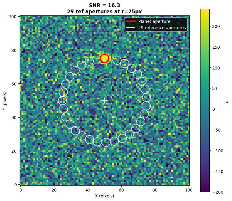
The snr() function places discrete apertures around the annulus at the planet’s separation. It uses the standard deviation of aperture fluxes as the noise estimate, with a small-sample correction for few apertures.

Reference: Mawet et al. (2014), ApJ, 792, 97

# Calculate SNR
positions = jnp.array([[planet_y, planet_x]])
snr_val = float(snr(image_jax, positions, fwhm)[0])

print(f"SNR: {snr_val:.2f}")

SNR: 16.27

# Visualize Mawet aperture placement using the actual geometry function
fig, ax = plt.subplots(figsize=(8, 8))

vmax = np.percentile(image, 99)
ax.imshow(image, origin='lower', cmap='viridis', vmin=-200, vmax=vmax)

# Calculate planet angle (same as used in the actual SNR calculation)
planet_angle = np.arctan2(planet_y - center, planet_x - center)

# Calculate number of apertures
n_apertures = calculate_n_apertures(radius=planet_sep, fwhm=fwhm)

# Generate aperture coords using the ACTUAL library function
y_coords, x_coords, mask = generate_aperture_coords(
    center=(center, center),
    radius=planet_sep,
    planet_angle=planet_angle,
    n_apertures=n_apertures,
    fwhm=fwhm
)

# Draw planet aperture in red
planet_circle = Circle((planet_x, planet_y), fwhm/2, fill=False, color='red', linewidth=3)
ax.add_patch(planet_circle)

# Draw reference apertures using the actual computed coordinates
y_arr = np.array(y_coords)
x_arr = np.array(x_coords)
mask_arr = np.array(mask)

for i in range(len(mask_arr)):
    if mask_arr[i]:
        circle = Circle((x_arr[i], y_arr[i]), fwhm/2, fill=False, 
                        color='white', linewidth=1.5, alpha=0.8)
        ax.add_patch(circle)

ax.scatter([center], [center], marker='+', s=200, color='white', linewidths=2)
ax.set_title(f'SNR = {snr_val:.1f}\n{n_apertures} ref apertures at r={planet_sep}px', 
             fontsize=12, fontweight='bold')
ax.set_xlabel('X (pixels)')
ax.set_ylabel('Y (pixels)')

# Legend
legend_elements = [
    Line2D([0], [0], color='red', linewidth=3, label='Planet aperture'),
    Line2D([0], [0], color='white', linewidth=1.5, label=f'{n_apertures} reference apertures')
]
ax.legend(handles=legend_elements, loc='upper right', facecolor='black', labelcolor='white')

plt.colorbar(ax.images[0], ax=ax, label='e-', shrink=0.8)
plt.tight_layout()
plt.show()

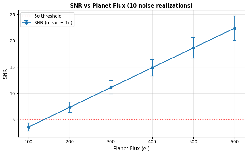
SNR vs Flux

SNR should scale linearly with planet flux. We average over multiple noise realizations to show the expected trend with error bars indicating statistical uncertainty.

# Measure SNR across different flux levels with multiple noise realizations
flux_values = np.array([100, 200, 300, 400, 500, 600])
n_realizations = 10

# Collect SNR samples for each flux
snr_samples = np.zeros((len(flux_values), n_realizations))

for i, flux in enumerate(flux_values):
    for j in range(n_realizations):
        np.random.seed(j)  # Different noise for each realization
        test_image = np.random.normal(0, noise_level, (size, size))
        test_image += flux * np.exp(-r2 / (2 * sigma**2))
        test_jax = jnp.array(test_image)
        snr_samples[i, j] = float(snr(test_jax, positions, fwhm)[0])

# Calculate mean and std
snr_mean = snr_samples.mean(axis=1)
snr_std = snr_samples.std(axis=1)

# Plot with error bars
fig, ax = plt.subplots(figsize=(8, 5))
ax.errorbar(flux_values, snr_mean, yerr=snr_std, fmt='o-', 
            label='SNR (mean ± 1σ)', color='tab:blue', 
            linewidth=2, capsize=4, capthick=1.5)
ax.axhline(y=5, color='red', linestyle=':', alpha=0.7, label='5σ threshold')

ax.set_xlabel('Planet Flux (e-)', fontsize=11)
ax.set_ylabel('SNR', fontsize=11)
ax.set_title(f'SNR vs Planet Flux ({n_realizations} noise realizations)', fontsize=12, fontweight='bold')
ax.legend()
ax.grid(alpha=0.3)
plt.tight_layout()
plt.show()

Using Estimators for Pipelines

For high-performance iterative pipelines, use snr_estimator() to pre-compute the aperture kernel:

import time

# Create estimator once
estimator = snr_estimator(fwhm, fast=True)

# Warmup (JIT compilation)
_ = estimator(image_jax, positions).block_until_ready()

# Time repeated calls
t0 = time.time()
for _ in range(100):
    estimator(image_jax, positions).block_until_ready()
elapsed = (time.time() - t0) / 100 * 1000

print(f"SNR Estimator: {elapsed:.2f} ms/call")

SNR Estimator: 1.54 ms/call

Summary

Function	Class	Use Case
snr()	SNREstimator	Mawet 2014 method - publications, detection claims

For iterative pipelines, use the estimator:

estimator = snr_estimator(fwhm, fast=True)  # Pre-compute kernel
snrs = estimator(image, positions)          # Fast repeated calls