Full Pipeline: coronagraphoto + coronalyze

This notebook demonstrates the complete workflow from image simulation to SNR calculation:

1. coronagraphoto generates simulated coronagraphic observations

2. coronalyze performs PSF subtraction and SNR analysis

We’ll demonstrate two SNR calculation approaches:

• snr_map: Generates a full 2D detection map (ideal for visualization)

• snr: Calculates SNR at specific positions (ideal for known targets)

import jax
import jax.numpy as jnp
import numpy as np
import matplotlib.pyplot as plt
from matplotlib.patches import Circle
import time

import coronalyze as cz

/home/docs/checkouts/readthedocs.org/user_builds/coronalyze/envs/latest/lib/python3.12/site-packages/tqdm/auto.py:21: TqdmWarning: IProgress not found. Please update jupyter and ipywidgets. See https://ipywidgets.readthedocs.io/en/stable/user_install.html
  from .autonotebook import tqdm as notebook_tqdm

Performance Comparison: snr vs snr_map

Both functions are JAX-compiled. The first call incurs a one-time compilation cost, but subsequent calls are extremely fast.

Method	Use Case	Complexity	Best For
snr()	Known positions	O(K)	Yield sims, pipelines
snr_map()	Full 2D map	O(N²)	Visualization, blind searches

# Create a test image for timing comparison
test_image = jnp.zeros((300, 300))
test_positions = jnp.array([[150.0, 150.0], [100.0, 100.0], [200.0, 200.0]])
fwhm_test = 4.0

# Time snr() - first call includes compilation
t0 = time.perf_counter()
_ = cz.snr(test_image, test_positions, fwhm_test).block_until_ready()
snr_compile_time = time.perf_counter() - t0

# Time snr() - reuse (after compilation)
t0 = time.perf_counter()
for _ in range(100):
    _ = cz.snr(test_image, test_positions, fwhm_test).block_until_ready()
snr_reuse_time = (time.perf_counter() - t0) / 100

# Time snr_map() - first call includes compilation  
t0 = time.perf_counter()
_ = cz.snr_map(test_image, fwhm_test).block_until_ready()
snr_map_compile_time = time.perf_counter() - t0

# Time snr_map() - reuse (after compilation)
t0 = time.perf_counter()
for _ in range(10):
    _ = cz.snr_map(test_image, fwhm_test).block_until_ready()
snr_map_reuse_time = (time.perf_counter() - t0) / 10

print("Performance Comparison (300x300 image, 3 positions):")
print(f"\nsnr() - 3 known positions:")
print(f"  First call (compile): {snr_compile_time*1000:.0f} ms")
print(f"  Subsequent calls:     {snr_reuse_time*1000:.2f} ms")
print(f"\nsnr_map() - full 90,000 pixel map:")
print(f"  First call (compile): {snr_map_compile_time*1000:.0f} ms")
print(f"  Subsequent calls:     {snr_map_reuse_time*1000:.0f} ms")
print(f"\nSpeedup ratio (snr vs snr_map): {snr_map_reuse_time/snr_reuse_time:.0f}x faster for known positions")

Performance Comparison (300x300 image, 3 positions):

snr() - 3 known positions:
  First call (compile): 760 ms
  Subsequent calls:     6.01 ms

snr_map() - full 90,000 pixel map:
  First call (compile): 1413 ms
  Subsequent calls:     753 ms

Speedup ratio (snr vs snr_map): 125x faster for known positions

Local test

Readthedocs doesn’t have the fastest machine, on my Macbook I get:

Performance Comparison (300x300 image, 3 positions):

snr() - 3 known positions:
  First call (compile): 6967 ms
  Subsequent calls:     17.43 ms

snr_map() - full 90,000 pixel map:
  First call (compile): 7833 ms
  Subsequent calls:     265 ms

Speedup ratio (snr vs snr_map): 15x faster for known positions

1. Download Example Data

coronalyze includes example data via pooch. The first time you run this, it will download:

• A coronagraph YIP (eac1_aavc_512 created by Susan Redmond)

• An ExoVista scene (modified Solar System)

# Fetch example data (downloads from GitHub if not cached)
coronagraph_path = cz.fetch_coronagraph()
scene_path = cz.fetch_scene()

print(f"Coronagraph: {coronagraph_path}")
print(f"Scene: {scene_path}")

Downloading file 'coronagraphs.zip' from 'https://github.com/CoreySpohn/coronalyze/raw/main/data/coronagraphs.zip' to '/home/docs/.cache/coronalyze'.

Unzipping contents of '/home/docs/.cache/coronalyze/coronagraphs.zip' to '/home/docs/.cache/coronalyze/coronagraphs.zip.unzip'

Downloading file 'scenes.zip' from 'https://github.com/CoreySpohn/coronalyze/raw/main/data/scenes.zip' to '/home/docs/.cache/coronalyze'.

Unzipping contents of '/home/docs/.cache/coronalyze/scenes.zip' to '/home/docs/.cache/coronalyze/scenes.zip.unzip'

Coronagraph: /home/docs/.cache/coronalyze/coronagraphs.zip.unzip/coronagraphs/eac1_aavc_512
Scene: /home/docs/.cache/coronalyze/scenes.zip.unzip/scenes/solar_system_mod.fits

2. Load Data with coronagraphoto and yippy

from yippy import Coronagraph as YippyCoronagraph
from coronagraphoto import (
    Exposure, OpticalPath, load_sky_scene_from_exovista
)
from coronagraphoto.optical_elements import (
    PrimaryAperture, SimpleDetector, ConstantThroughputElement, from_yippy
)
from coronagraphoto.core.simulation import sim_star, sim_planets, sim_disk, sim_zodi

# Load scene and coronagraph
scene = load_sky_scene_from_exovista(scene_path)
yippy_coro = YippyCoronagraph(coronagraph_path, use_jax=True, use_quarter_psf_datacube=True)
coronagraph = from_yippy(yippy_coro)

print(f"Loaded scene with {scene.planets.n_planets} planets")

[yippy] INFO [2026-02-24 00:47:56,304] Creating eac1_aavc_512 coronagraph

[yippy] WARNING [2026-02-24 00:47:56,306] Unhandled header fields: {'TMULCHAR', 'TMULDET', 'D_INSC'}

[yippy] WARNING [2026-02-24 00:47:56,307] Using default unit for D: m. Could not extract unit from comment: "circumscribed diameter of the telescope in mete"

[yippy] INFO [2026-02-24 00:47:56,334] eac1_aavc_512 is quarterly symmetric

[yippy] WARNING [2026-02-24 00:47:56,592] 2d contrast/throughput not supported currently

[yippy] INFO [2026-02-24 00:47:56,593] Created eac1_aavc_512

Loaded scene with 8 planets

3. Setup

optical_path = OpticalPath(
    primary=PrimaryAperture(diameter_m=6.0),
    attenuating_elements=(ConstantThroughputElement(throughput=0.9),),
    coronagraph=coronagraph,
    detector=SimpleDetector(pixel_scale=1/512, shape=(300, 300))
)

# Calculate FWHM from the coronagraph pixel scale
# FWHM of Airy disk ≈ 1.03 λ/D, and pixel_scale_lod = (λ/D)/pixel
fwhm = 1.03 / coronagraph.pixel_scale_lod

print(f"Coronagraph pixel scale: {coronagraph.pixel_scale_lod:.4f} (λ/D)/pixel")
print(f"Calculated FWHM: {fwhm:.2f} pixels")

Coronagraph pixel scale: 0.2500 (λ/D)/pixel
Calculated FWHM: 4.12 pixels

4. Simulate Observation with coronagraphoto

We simulate the star and planets separately, which allows us to have both:

• A noisy observation (star + planets + noise)

• A noiseless stellar model for perfect subtraction

from coronagraphoto import conversions

# Define exposure
exposure = Exposure(
    start_time_jd=conversions.decimal_year_to_jd(2001.25),
    exposure_time_s=24*3600.0,  # 1 day
    central_wavelength_nm=jnp.array([550.0]),
    bin_width_nm=jnp.array([100.0]),
    position_angle_deg=0.0
)

# Simulate each component
key = jax.random.PRNGKey(0)
k1, k2, k3, k4 = jax.random.split(key, 4)

args = (
    exposure.start_time_jd, 
    exposure.exposure_time_s,
    exposure.central_wavelength_nm[0], 
    exposure.bin_width_nm[0]
)

star_electrons = sim_star(*args, scene.stars, optical_path, k1)
planet_electrons = sim_planets(*args, exposure.position_angle_deg, scene.planets, optical_path, k2)

# Full observation = star + planets
observation = star_electrons + planet_electrons

# Add detector noise
noise_electrons = optical_path.detector.readout_noise_electrons(exposure.exposure_time_s, key)
noisy_observation = observation + noise_electrons

fig, ax = plt.subplots()
ax.imshow(noisy_observation, origin='lower', cmap='magma')
ax.set_title("Observation")
ax.set_xlabel("x (pixels)")
ax.set_ylabel("y (pixels)")
plt.show()

print(f"Observation shape: {noisy_observation.shape}")
print(f"Max signal: {float(jnp.max(noisy_observation)):.1f} e-")

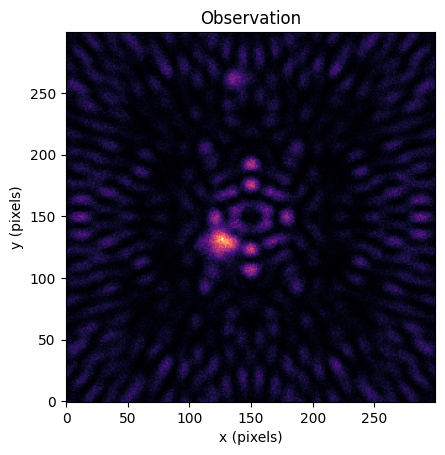
Observation shape: (300, 300)
Max signal: 122.0 e-

5. PSF Subtraction with coronalyze

With coronagraphoto, we have the noiseless stellar expectation - this enables perfect PSF subtraction.

# Get noiseless stellar expectation for perfect subtraction
star_expectation = sim_star(*args, scene.stars, optical_path, jax.random.PRNGKey(0))

# Perfect PSF subtraction
residual = cz.subtract_star(noisy_observation, star_expectation)

print(f"Residual mean: {float(jnp.mean(residual)):.2f} e-")
print(f"Residual std: {float(jnp.std(residual)):.2f} e-")

Residual mean: 0.50 e-

Residual std: 4.64 e-

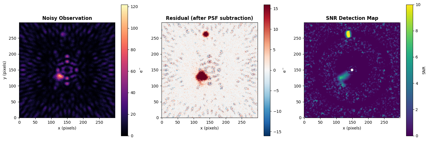
6. SNR Analysis: Method 1 - SNR Map

The snr_map function generates a full 2D detection map. This is ideal for:

• Visualization

• Blind searches

• Understanding the detection landscape

# Generate full SNR detection map
snr_detection_map = cz.snr_map(residual, fwhm)

print(f"SNR map shape: {snr_detection_map.shape}")
print(f"Max SNR in map: {float(jnp.nanmax(snr_detection_map)):.1f}")

SNR map shape: (300, 300)

Max SNR in map: 24.3

# Plot the observation, residual, and SNR map side by side
fig, axes = plt.subplots(1, 3, figsize=(15, 5))

# Raw observation
im0 = axes[0].imshow(noisy_observation, origin='lower', cmap='magma')
axes[0].set_title('Noisy Observation', fontsize=12, fontweight='bold')
axes[0].set_xlabel('x (pixels)')
axes[0].set_ylabel('y (pixels)')
plt.colorbar(im0, ax=axes[0], label='e$^-$')

# Residual after PSF subtraction
vmax = float(jnp.nanpercentile(jnp.abs(residual), 99))
im1 = axes[1].imshow(residual, origin='lower', cmap='RdBu_r', vmin=-vmax, vmax=vmax)
axes[1].set_title('Residual (after PSF subtraction)', fontsize=12, fontweight='bold')
axes[1].set_xlabel('x (pixels)')
plt.colorbar(im1, ax=axes[1], label='e$^-$')

# SNR detection map
im2 = axes[2].imshow(snr_detection_map, origin='lower', cmap='viridis', vmin=0, vmax=10)
axes[2].set_title('SNR Detection Map', fontsize=12, fontweight='bold')
axes[2].set_xlabel('x (pixels)')
plt.colorbar(im2, ax=axes[2], label='SNR')

plt.tight_layout()
plt.show()

7. SNR Analysis: Method 2 - Known Positions

When you know the planet positions (e.g., from orbital predictions), the snr function is much faster.

This is the preferred method for:

• Yield simulations

• Follow-up observations

• Performance-critical pipelines

# Get actual planet positions from the scene
planet_pos_arcsec = scene.planets.position(exposure.start_time_jd)  # (2, n_planets)

# Convert from arcsec to pixels
pixel_scale = optical_path.detector.pixel_scale  # arcsec/pixel
center = (noisy_observation.shape[0] - 1) / 2.0

# Position format is (dRA, dDec) -> convert to (y, x) pixel coords
planet_x = center + planet_pos_arcsec[0] / pixel_scale
planet_y = center + planet_pos_arcsec[1] / pixel_scale
planet_positions = jnp.stack([planet_y, planet_x], axis=1)  # (n_planets, 2)

print(f"Number of planets: {planet_positions.shape[0]}")
print(f"Planet positions (y, x):")
for i, pos in enumerate(planet_positions):
    print(f"  Planet {i}: ({float(pos[0]):.1f}, {float(pos[1]):.1f})")

Number of planets: 8
Planet positions (y, x):
  Planet 0: (149.7, 160.6)
  Planet 1: (130.6, 127.8)
  Planet 2: (125.5, 116.8)
  Planet 3: (107.2, 121.6)
  Planet 4: (261.8, 137.5)
  Planet 5: (388.9, 213.4)
  Planet 6: (253.9, 824.8)
  Planet 7: (81.9, 1032.5)

# Calculate SNR at known positions
snr_values = cz.snr(residual, planet_positions, fwhm)

print("\nSNR values at planet positions:")
for i, snr_val in enumerate(snr_values):
    print(f"  Planet {i}: SNR = {float(snr_val):.2f}")

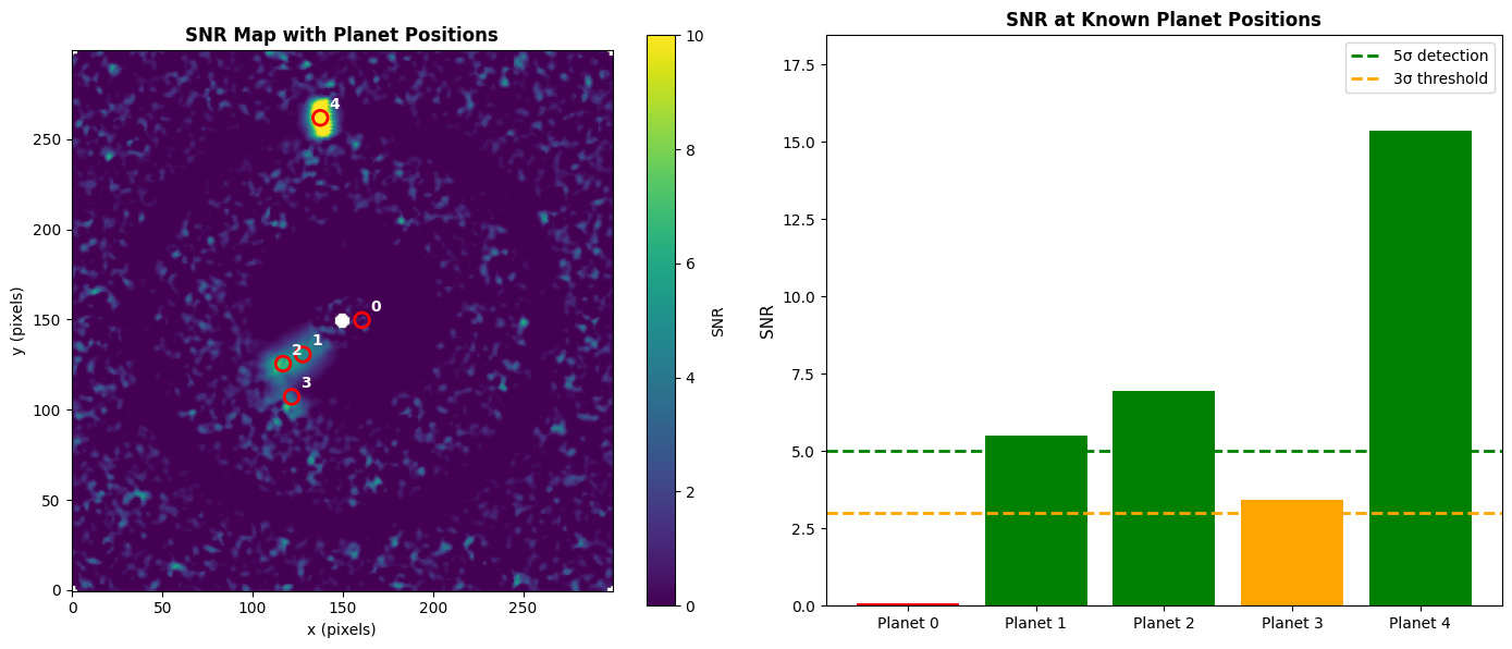
SNR values at planet positions:
  Planet 0: SNR = 0.09
  Planet 1: SNR = 5.51
  Planet 2: SNR = 6.95
  Planet 3: SNR = 3.43
  Planet 4: SNR = 15.38
  Planet 5: SNR = nan
  Planet 6: SNR = nan
  Planet 7: SNR = nan

8. Visualization: Comparing Both Methods

Let’s overlay the known planet positions on the SNR map to compare the two approaches.

fig, axes = plt.subplots(1, 2, figsize=(14, 6))

# Left: SNR map with planet positions marked
im0 = axes[0].imshow(snr_detection_map, origin='lower', cmap='viridis', vmin=0, vmax=10)
for i, pos in enumerate(planet_positions):
    # Only show planets within the image bounds
    if 0 <= pos[0] < 300 and 0 <= pos[1] < 300:
        circle = Circle((float(pos[1]), float(pos[0])), fwhm, 
                        fill=False, color='red', linewidth=2)
        axes[0].add_patch(circle)
        axes[0].annotate(f'{i}', (float(pos[1])+5, float(pos[0])+5), 
                        color='white', fontsize=10, fontweight='bold')
axes[0].set_title('SNR Map with Planet Positions', fontsize=12, fontweight='bold')
axes[0].set_xlabel('x (pixels)')
axes[0].set_ylabel('y (pixels)')
plt.colorbar(im0, ax=axes[0], label='SNR')

# Right: Bar chart comparing SNR values
# Filter to planets within the image
valid_indices = []
valid_snrs = []
for i, (pos, snr_val) in enumerate(zip(planet_positions, snr_values)):
    if 0 <= pos[0] < 300 and 0 <= pos[1] < 300:
        valid_indices.append(i)
        valid_snrs.append(float(snr_val))

colors = ['green' if s >= 5 else 'orange' if s >= 3 else 'red' for s in valid_snrs]
bars = axes[1].bar([f'Planet {i}' for i in valid_indices], valid_snrs, color=colors)
axes[1].axhline(y=5, color='green', linestyle='--', linewidth=2, label='5σ detection')
axes[1].axhline(y=3, color='orange', linestyle='--', linewidth=2, label='3σ threshold')
axes[1].set_ylabel('SNR', fontsize=11)
axes[1].set_title('SNR at Known Planet Positions', fontsize=12, fontweight='bold')
axes[1].legend(loc='upper right')
axes[1].set_ylim(0, max(valid_snrs) * 1.2 if valid_snrs else 10)

plt.tight_layout()
plt.show()

Summary

Both methods use the same underlying Mawet et al. (2014) small-sample statistics, so they produce identical results at the same positions.

Choose snr() for known positions in yield simulations or performance-critical pipelines.

Choose snr_map() for visualization, blind searches, or understanding the detection landscape.