Quick Start

This notebook demonstrates the basic usage of coronalyze for SNR calculation.

import jax.numpy as jnp
import numpy as np
import matplotlib.pyplot as plt
from matplotlib.patches import Patch
import time

import coronalyze as cz
from coronalyze.core.geometry import calculate_n_apertures, generate_aperture_coords

/home/docs/checkouts/readthedocs.org/user_builds/coronalyze/envs/latest/lib/python3.12/site-packages/tqdm/auto.py:21: TqdmWarning: IProgress not found. Please update jupyter and ipywidgets. See https://ipywidgets.readthedocs.io/en/stable/user_install.html
  from .autonotebook import tqdm as notebook_tqdm

Creating a Test Image

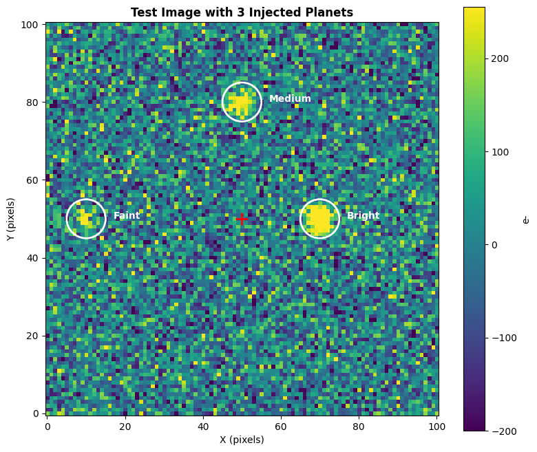
Let’s create a simple test image with planets and noise to demonstrate SNR calculation.

# Image parameters
size = 101
fwhm = 5.0
noise_level = 100.0
center = size // 2

# Create noise background
np.random.seed(0)
image = np.random.normal(0, noise_level, (size, size))

# Add planets at different separations and fluxes
planets = [
    {'sep': 20, 'angle': 0, 'flux': 800, 'label': 'Bright'},
    {'sep': 30, 'angle': 90, 'flux': 400, 'label': 'Medium'},
    {'sep': 40, 'angle': 180, 'flux': 200, 'label': 'Faint'},
]

sigma = fwhm / 2.355
y, x = np.ogrid[:size, :size]

planet_positions = []
for p in planets:
    angle_rad = np.radians(p['angle'])
    py = center + p['sep'] * np.sin(angle_rad)
    px = center + p['sep'] * np.cos(angle_rad)
    planet_positions.append((py, px))
    r2 = (y - py)**2 + (x - px)**2
    image += p['flux'] * np.exp(-r2 / (2 * sigma**2))

image_jax = jnp.array(image)

# Visualize the test image
fig, ax = plt.subplots(figsize=(8, 8))

vmax = np.percentile(image, 99)
im = ax.imshow(image, origin='lower', cmap='viridis', vmin=-200, vmax=vmax)
plt.colorbar(im, ax=ax, label='e-', shrink=0.8)

# Mark planets with high-contrast white circles
for i, ((py, px), p) in enumerate(zip(planet_positions, planets)):
    circle = plt.Circle((px, py), fwhm, fill=False, color='white', linewidth=2)
    ax.add_patch(circle)
    ax.annotate(p['label'], (px + fwhm + 2, py), color='white', fontsize=10, fontweight='bold')

# Mark center
ax.scatter([center], [center], marker='+', s=150, color='red', linewidths=2)

ax.set_title('Test Image with 3 Injected Planets', fontsize=12, fontweight='bold')
ax.set_xlabel('X (pixels)')
ax.set_ylabel('Y (pixels)')
plt.tight_layout()
plt.show()

Calculating SNR

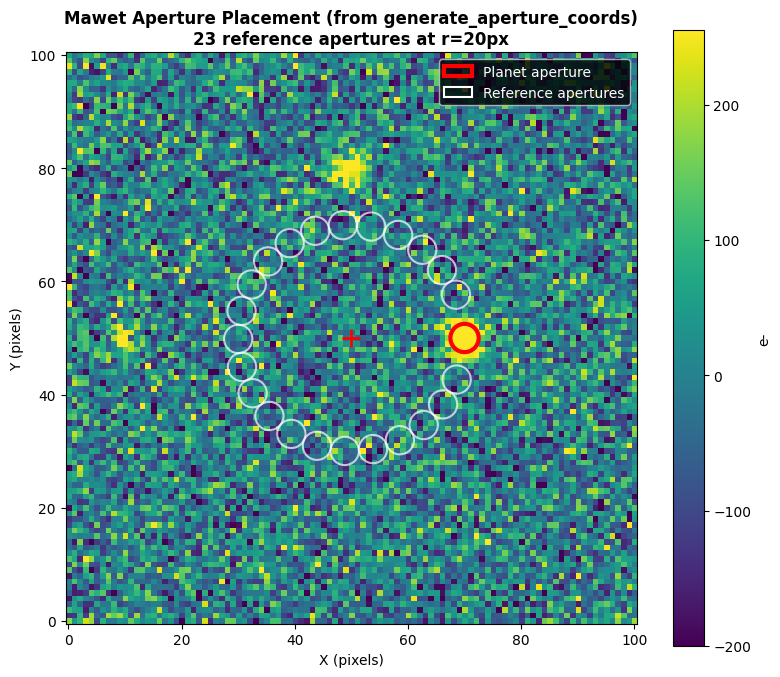
The SNR calculations use the method from Mawet et al. (2014) which places apertures around the planet’s radius to estimate background statistics.

Use cz.snr() for batch calculations:

# Convert positions to array format (N, 2) with (y, x) coordinates
positions_array = jnp.array(planet_positions)

# Calculate SNR for all planets at once
snrs = cz.snr(image_jax, positions_array, fwhm)

print(f"{'Planet':<20} {'SNR':>8}")
print("-" * 30)

for snr_val, p in zip(snrs, planets):
    print(f"{p['label']:<20} {float(snr_val):>8.1f}")

Planet                    SNR
------------------------------
Bright                   30.6
Medium                   11.4
Faint                     7.8

Visualizing the SNR Method

The Mawet SNR method places non-overlapping apertures at the same separation to estimate background noise.

We use generate_aperture_coords from the coronalyze.core library to visualize the actual apertures used in the calculation:

# Visualize aperture placement for the bright planet
py, px = planet_positions[0]  # Bright planet
sep = planets[0]['sep']

# Calculate planet angle (same as used in the actual SNR calculation)
planet_angle = np.arctan2(py - center, px - center)

# Calculate number of apertures
n_apertures = calculate_n_apertures(radius=sep, fwhm=fwhm)

# Generate aperture coords using the actual library function
y_coords, x_coords, mask = generate_aperture_coords(
    center=(center, center),
    radius=sep,
    planet_angle=planet_angle,
    n_apertures=n_apertures,
    fwhm=fwhm
)

fig, ax = plt.subplots(figsize=(8, 8))
im = ax.imshow(image, origin='lower', cmap='viridis', vmin=-200, vmax=vmax)
plt.colorbar(im, ax=ax, label='e-', shrink=0.8)

# Draw planet aperture in red
planet_circle = plt.Circle((px, py), fwhm/2, fill=False, color='red', linewidth=3)
ax.add_patch(planet_circle)

# Draw reference apertures using the actual computed coordinates
y_arr = np.array(y_coords)
x_arr = np.array(x_coords)
mask_arr = np.array(mask)

for i in range(len(mask_arr)):
    if mask_arr[i]:
        circle = plt.Circle((x_arr[i], y_arr[i]), fwhm/2, fill=False, 
                            color='white', linewidth=1.5, alpha=0.7)
        ax.add_patch(circle)

ax.scatter([center], [center], marker='+', s=150, color='red', linewidths=2)
ax.set_title(f'Mawet Aperture Placement (from generate_aperture_coords)\n{n_apertures} reference apertures at r={sep}px', 
             fontsize=12, fontweight='bold')
ax.set_xlabel('X (pixels)')
ax.set_ylabel('Y (pixels)')

# Legend
legend_elements = [
    Patch(facecolor='none', edgecolor='red', linewidth=3, label='Planet aperture'),
    Patch(facecolor='none', edgecolor='white', linewidth=1.5, label='Reference apertures')
]
ax.legend(handles=legend_elements, loc='upper right', facecolor='black', labelcolor='white')

plt.tight_layout()
plt.show()

Using the Estimator API for Pipelines

For high-performance pipelines, use snr_estimator() to pre-compute the kernel once:

# Create an estimator (pre-computes the aperture kernel)
estimator = cz.snr_estimator(fwhm, fast=True)

# Warm up JIT
_ = estimator(image_jax, positions_array).block_until_ready()
_ = cz.snr(image_jax, positions_array, fwhm).block_until_ready()

# Time convenience function
t0 = time.time()
for _ in range(100):
    cz.snr(image_jax, positions_array, fwhm).block_until_ready()
convenience_time = (time.time() - t0) / 100 * 1000

# Time estimator
t0 = time.time()
for _ in range(100):
    estimator(image_jax, positions_array).block_until_ready()
estimator_time = (time.time() - t0) / 100 * 1000

print(f"snr() convenience:   {convenience_time:.2f} ms")
print(f"estimator() reuse:   {estimator_time:.2f} ms")
print(f"Speedup:             {convenience_time/estimator_time:.1f}x")

snr() convenience:   1.69 ms
estimator() reuse:   1.59 ms
Speedup:             1.1x

Next Steps

For a complete pipeline with realistic stellar speckle subtraction, see the coronagraphoto integration notebook.